Week 9 FAQs
📚 Topics Covered in Week 9
- Linear Separability
- Perceptron
- Logistic Regression
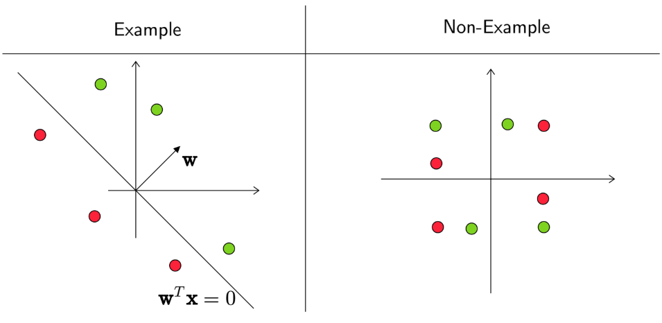
🔍 Linear Separability
A dataset is considered linearly separable if there exists a linear classifier that can perfectly distinguish all data points, resulting in zero training error. Mathematically, for a dataset:
\[ D = \left\{ (\mathbf{x}_1, y_1),\cdots, (\mathbf{x}_n,y_n) \right\} \]
there exists a weight vector \(\mathbf{w}\) such that:
\[ (\mathbf{w}^T\mathbf{x_i})y_i \geq 0 \quad \forall i \]
where \(y_i \in \{1, -1\}\).
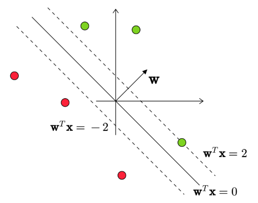
Linear Separability with Margin \(\gamma\)
If a dataset is separable with a positive margin \(\gamma\), then there exists a weight vector \(\mathbf{w}\) and \(\gamma > 0\) such that:
\[ (\mathbf{w}^T\mathbf{x_i})y_i \geq \gamma \quad \forall i \]
where \(y_i \in \{1, -1\}\).
🔍 Perceptron
Prediction in Perceptron
The Perceptron algorithm makes predictions using the following rule:
\[ \hat{y} = \begin{cases} 1 & \mathbf{w}^{T}\mathbf{x} \geqslant 0\\ -1 & \mathbf{w}^{T}\mathbf{x} < 0 \end{cases} \]
In this course, we follow the convention that \(\mathbf{w}^{T}\mathbf{x} = 0\) is predicted as 1.
Perceptron Algorithm Steps
Initialize the weight vector (\(\mathbf{w}\)). If unspecified, it is typically initialized as \(\mathbf{w} = 0\).
Iterate through the dataset in a fixed order (not necessarily sequential).
Update the weights if a misclassification occurs:
If the algorithm makes a mistake on the \(i^{th}\) data point, update the weight vector as:
\[ \mathbf{w}^{t+1} = \mathbf{w}^{t} + \mathbf{x}_i y_i \]
Termination: The algorithm stops once it completes \(n\) consecutive iterations without errors.
Proof of Convergence
If the dataset is linearly separable with a positive margin.
If there exists some \(R > 0\) such that:
\[ \|\mathbf{x}_i\|^2 \leq R^2 \quad \forall i \]
Then, we derive the following bounds:
Upper Bound:
\[ \|\mathbf{w}^{t}\|^2 \leq t \cdot R^2 \]
Lower Bound:
\[ \|\mathbf{w}^{t}\|^2 \geq t^2 \cdot \gamma^2 \]
Radius-Margin Bound:
\[ t \leq \frac{R^2}{\gamma^2} \]
This means that the Perceptron algorithm makes at most \(\frac{R^2}{\gamma^2}\) mistakes, ensuring convergence.
Key Observations About Perceptron
- Even for linearly separable data, multiple solutions exist, and the final solution depends on initialization and the order of data points.
- If the data is not linearly separable, the perceptron algorithm never converges.
- Outliers significantly impact the Perceptron algorithm. Since weight updates occur only for misclassified points, an outlier can lead to large weight changes, reducing generalization.
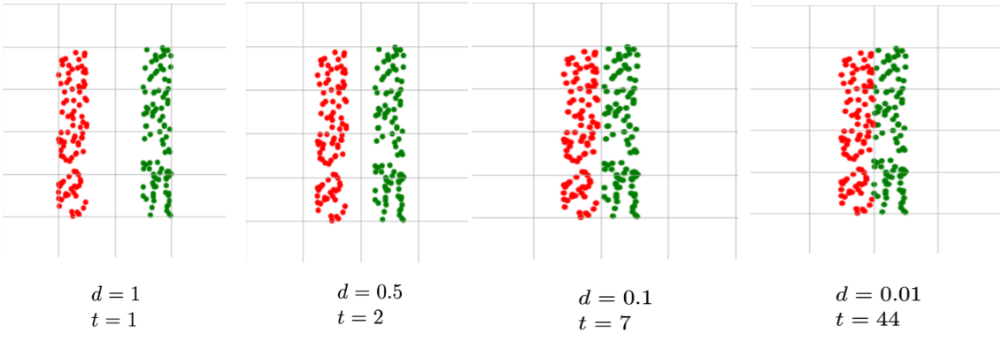
- Smaller margin increases the number of updates, meaning that perceptron requires more iterations to converge.
🔍 Logistic Regression
Sigmoid Function
The sigmoid function \(g(z)\), also called the logistic function, is defined as:
\[ g(z) = \frac{1}{1+e^{-z}} \]
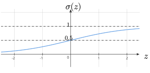
Properties:
The function outputs values between 0 and 1.
\(\sigma(0) = 0.5\).
\(\sigma(-z) = 1 - \sigma(z)\).
If \(z > 0\), then \(\sigma(z) > 0.5\); if \(z < 0\), then \(\sigma(z) < 0.5\).
The derivative is:
\[ \frac{d \sigma}{d z} = \sigma(z)(1-\sigma(z)) \]
Probability of Prediction in Logistic Regression
The probability of \(y = 1\) given input \(\mathbf{x}\) is modeled as:
\[ P(y=1 \mid \mathbf{x}) = \sigma(\mathbf{w}^T \mathbf{x}) \]
where \(\sigma\) is the sigmoid function. This relaxes the assumption of strict linear separability.
The classifier is defined as:
\[ \hat{y} = \begin{cases} 1 & \sigma \left(\mathbf{w}^{T}\mathbf{x}\right) \geqslant T\\ 0 & \sigma \left(\mathbf{w}^{T}\mathbf{x}\right) < T \end{cases} \]
where \(T\) is a threshold value determined by the problem. The decision boundary is given by:
\[ \sigma(\mathbf{w}^T \mathbf{x}) = T \]
Simplifying:
\[ \mathbf{w}^T \mathbf{x} = -\ln\left(\frac{1}{T}-1\right) \]
Maximum Likelihood Estimation (MLE) for Logistic Regression
The probability of \(y_i\) given data point \(\mathbf{x}_i\) is:
\[ P(y_i \mid \mathbf{x}_i) = \sigma_i^{y_i} \cdot (1-\sigma_i)^{1-y_i} \]
where \(\sigma_i = P(y_i=1 \mid \mathbf{x}_i) = \sigma(\mathbf{w}^T\mathbf{x})\).
Likelihood Function:
\[ \mathbf{L}(\mathbf{w}; D) = \prod_{i=1}^{n} P(y_i \mid \mathbf{x}_i;\mathbf{w} ) = \prod_{i=1}^{n}\sigma_i^{y_i} \cdot (1-\sigma_i)^{1-y_i} \]
Log-Likelihood:
\[ \sum_{i=1}^{n} y_i \log[\sigma(\mathbf{w}^T \mathbf{x})] + (1-y_i)\log[1-\sigma(\mathbf{w}^T \mathbf{x})] \]
Cross-Entropy Loss
The negative log-likelihood serves as the loss function:
\[ \sum_{i=1}^{n} -y_i \log[\sigma(\mathbf{w}^T \mathbf{x})] -(1-y_i)\log[1-\sigma(\mathbf{w}^T \mathbf{x})] \]
Gradient of MLE
The gradient of the likelihood function is:
\[ \sum_{i=1}^{n} (y_i - \sigma_i)\mathbf{x}_i \]
where \((y_i - \sigma_i)\) represents the error in prediction.
Key Observations
- Logistic regression does not require data to be linearly separable.
- As \(\mathbf{w}^{T}\mathbf{x} \to \infty\), the predicted probability approaches 1.
- The concept extends to multi-class classification using the softmax function.
💡 Need Assistance?
For any queries, feel free to reach out via email:
📧 22f3001839@ds.study.iitm.ac.in