Week 1 FAQs
📚 Topics Covered in Week 1
- Principal Component Analysis (PCA)
- PCA is a technique used for dimensionality reduction by projecting data into a lower-dimensional space while preserving as much variance as possible.
- Reconstruction Error
- Measures how well the data is represented by its projected form. Various forms of reconstruction error are explored in the course.
- Eigenvectors and Eigenvalues
- Understanding the relationship between data variance and the direction of eigenvectors, and how to compute variance in principal components.
- Total Variance and Top \(k\) Components
- Learn how to compute the total variance of the dataset and how to use the top \(k\) principal components to approximate the variance.
🔍 Projection
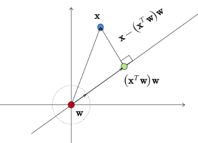
Vector Projection
The projection of \(\mathbf{x}_i\) onto \(\mathbf{w}\) is given by:
\[ \frac{(\mathbf{x}_i^T \mathbf{w}) \mathbf{w}}{\|\mathbf{w}\|^2} \]
If \(\|\mathbf{w}\| = 1\), this simplifies to:
\[ (\mathbf{x}_i^T \mathbf{w}) \mathbf{w} \]
Scalar Projection
The scalar projection is:
\[ \mathbf{x}_i^T \mathbf{w} \]
Projection onto Top \(k\) Principal Components
For top \(k\) components, the projection is:
\[ \tilde{\mathbf{x}} = (\mathbf{x}_i^T \mathbf{w}_1) \mathbf{w}_1 + \cdots + (\mathbf{x}_i^T \mathbf{w}_k) \mathbf{w}_k \]
🔍 Reconstruction Error Formula
The reconstruction error formula is given by:
\[ \frac{1}{n}\sum _{i=1}^{n} \| \mathbf{x}_i - \tilde{\mathbf{x}}_i \| ^{2} \]
Where:
- \(\mathbf{x}_i\) is the data point.
- \(\tilde{\mathbf{x}}_i\) is the projected data point.
Other Forms of Reconstruction Error
- Euclidean distance-based error:
\[ \frac{1}{n}\sum _{i=1}^{n} \| \mathbf{x}_i - \tilde{\mathbf{x}}_i \| ^{2} \]
- Inner product-based error:
\[ \frac{1}{n}\sum _{i=1}^{n} \left[\mathbf{x}_i - \tilde{\mathbf{x}}_i\right]^T \left[\mathbf{x}_i - \tilde{\mathbf{x}}_i\right] \]
- Component-wise error:
\[ \frac{1}{n}\left[\mathbf{x}_{i}^T \mathbf{x}_{i} - \left(\mathbf{x}_i^T \mathbf{w}\right)^2\right] \]
where \(\mathbf{w}\) is the vector of principal components.
🔍 Variance in the Direction of an Eigenvector
The variance in the direction of an eigenvector is calculated as:
\[ \frac{1}{n}\sum _{i=1}^{n} \left(\mathbf{x}_i^T \mathbf{w}\right)^2 = \frac{1}{n}\sum _{i=1}^{n} \mathbf{w}^T \mathbf{x}_i \mathbf{x}_i^T \mathbf{w} = \mathbf{w}^T C \mathbf{w} = \lambda \]
where \((\lambda, \mathbf{w})\) is the eigenpair of the covariance matrix \(C\).
🔍 Total Variance of the Dataset
The total variance of the dataset is given by:
\[ \sum _{i=1}^{d} \lambda_i \]
where \(\lambda_i\) represents the eigenvalue of the covariance matrix \(C\).
🔍 Variance Using Top \(k\) Principal Components
The proportion of variance explained by the top \(k\) principal components is:
\[ \frac{\sum _{i=1}^{k} \lambda_i}{\sum _{i=1}^{d} \lambda_i} \]
where \(\lambda_i\) is the eigenvalue of the covariance matrix \(C\).
Note: Ensure to sort the eigenvalues in descending order.
💡 Need Help?
For any technical issues or errors, please contact:
📧 22f3001839@ds.study.iitm.ac.in