Week 10 FAQs

📚 Topics Covered in Week 10

• Maximizing Margin
• Hard Margin Support Vector Machine (SVM)
• Kernel Trick

---

📺 Watch This First! 📺

Before diving into the FAQs, check out this tutorial! It provides a clear and concise explanation of the key concepts covered in Week 10, including margin maximization and SVM optimization. Watching this will help you grasp the fundamentals more effectively and make the FAQs easier to follow.

Hit play ▶️ and get started!

---

🔍 Maximizing Margin

Why Maximize Margin?

1. A larger margin improves generalization.
2. In perceptron learning, the model makes at most \(\frac{R^2}{\gamma^2}\) mistakes, where \(\gamma\) is the margin. A larger margin reduces the number of mistakes and iterations required for learning.
3. The prediction rule of a linear classifier depends on which side of the decision boundary a data point lies. If a data point is farther from the boundary, we can classify it with higher confidence, emphasizing the importance of maximizing the margin.

Geometric Margin

Geometric Margin

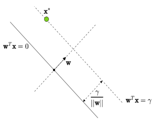
The distance between the decision boundary \(\mathbf{w}^T \mathbf{x} = 0\) and the margin hyperplane \(\mathbf{w}^T \mathbf{x} = \gamma\) is given by:

\[ \frac{\mathbf{w}^T \mathbf{x}^*}{\|\mathbf{w}\|} = \frac{\gamma}{\|\mathbf{w}\|} \]

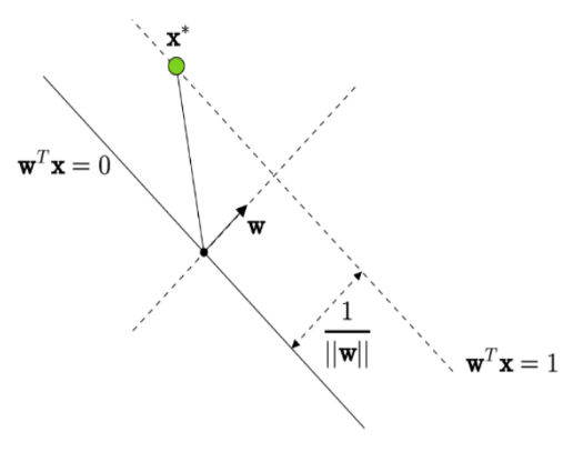
Since both \(\mathbf{w}\) and \(\gamma\) can be scaled without affecting the setup, we set \(\gamma = 1\), making the geometric margin:

\[ \frac{1}{\|\mathbf{w}\|} \]

Remark: \(\frac{1}{\|\mathbf w\|}\) is the geometric margin betwen \(\mathbf w^T \mathbf x =0\) and \(\mathbf w^T \mathbf x =\gamma\) while \(\gamma\) is the functional margin.

Note: The distance between any two hyperplanes \(\mathbf{w}^T \mathbf{x} = c_1\) and \(\mathbf{w}^T \mathbf{x} = c_2\) is:

\[ \frac{|c_1 - c_2|}{\|\mathbf{w}\|} \]

---

🔍 Hard Margin Support Vector Machine (SVM)

Optimization Problem

\[ \min_{\mathbf{w}} \frac{\| \mathbf{w} \| ^{2}}{2}, \quad \text{subject to} \quad (\mathbf{w}^{T}\mathbf{x}_{i}) y_{i} \geq 1,\ 1 \leq i \leq n \]

Using the Lagrangian function with multipliers \(\alpha_i\):

\[ \frac{\| \mathbf{w} \| ^{2}}{2} + \sum _{i=1}^{n} \alpha _{i}\left[ 1-(\mathbf{w}^{T}\mathbf{x}_{i}) y_{i}\right] \]

Primal Problem

The primal formulation seeks to minimize the objective function while ensuring that all constraints are satisfied. It is given by:

\[ \underset{\mathbf{w}}{\min} \ \underset{\alpha \geqslant 0}{\max} \ \frac{\| \mathbf{w} \| ^{2}}{2} + \sum _{i=1}^{n} \alpha _{i}\left[ 1-\left(\mathbf{w}^{T}\mathbf{x}_{i}\right) y_{i}\right] \]

Here, the optimization variable is \(\mathbf{w}\).

Dual Problem

The dual formulation flips the order of optimization, first minimizing over \(\mathbf{w}\) and then maximizing over \(\alpha\). This leads to:

\[ \underset{\alpha \geqslant 0}{\max} \ \underset{\mathbf{w}}{\min} \ \frac{\| \mathbf{w} \| ^{2}}{2} + \sum _{i=1}^{n} \alpha _{i}\left[ 1-\left(\mathbf{w}^{T}\mathbf{x}_{i}\right) y_{i}\right] \]

Here, the optimization variable is \(\alpha\). The dual problem is often preferred due to its simpler constraints and ability to incorporate kernel methods.

Dual Formulation

By setting the gradient to zero, we get:

\[ \mathbf{w} = \sum _{i=1}^{n} \alpha _{i}\mathbf{x}_{i} y_{i} \]

In matrix notation:

\[ \mathbf{w} = \mathbf{XY\alpha} \]

where:

\[ \mathbf{X} = \begin{bmatrix} | & & | \\\mathbf{x}_{1} & \cdots & \mathbf{x}_{n} \\\ | & & | \end{bmatrix}, \quad \mathbf{Y} = \begin{bmatrix} y_{1} & & \\\ & \ddots & \\\ & & y_{n} \end{bmatrix}, \quad \mathbf{\alpha} = \begin{bmatrix} \alpha _{1} \\\ \vdots \\\ \alpha _{n} \end{bmatrix} \]

Plugging into the dual objective:

\[ \max_{\alpha \geq 0} \quad \mathbf{\alpha }^{T}\mathbf{1} - \frac{1}{2} \mathbf{\alpha }^{T} (\mathbf{Y}^{T}\mathbf{X}^{T}\mathbf{XY}) \mathbf{\alpha} \]

Support Vectors

Support vectors are data points for which \(\alpha^* > 0\). They are crucial in defining the decision boundary.

Few key observations about support vectors:

1. Support vectors always lie on one of the two supporting hyperplanes: \((\mathbf{w}^{*})^{T}\mathbf{x}_{i} = \pm 1\).
2. Any point that is not on a supporting hyperplane has \(\alpha^*_i = 0\).
3. Not all points on the supporting hyperplane are necessarily support vectors.
4. If \(\alpha_i^* > 0\), the corresponding data point lies exactly on the hyperplane.
5. If \(\alpha_i^* = 0\), the data point satisfies the condition \(\mathbf{w}^T \mathbf{x}_i \geq 1\), meaning it is correctly classified and does not influence the margin.
6. Support vectors play a crucial role in defining the decision boundary, as they are the only points that impact the model’s parameters.

Ignore the bias term in this image, as it has not been covered in our course. Source: Stanford.edu

Prediction Rule

\[ \hat{y} = \begin{cases} 1, & \mathbf{w}^{T}\mathbf{x}_{\text{test}} \geq 0 \\ 0, & \mathbf{w}^{T}\mathbf{x}_{\text{test}} < 0 \end{cases} \]

---

🔍 Kernel Trick

A comparison between linear and kernel SVM:

	Linear SVM	Kernel SVM
Feature Mapping	\(\mathbf{x}_i\)	\(\phi(\mathbf{x}_i)\)
Data Matrix	\(\mathbf{X}\)	\(\phi(\mathbf{X})\)
Gram Matrix	\(\mathbf{X}^T\mathbf{X}\)	\(\mathbf{K}\)
Optimization Objective	\[\max_{\boldsymbol{\alpha} \geq 0} \quad \boldsymbol{\alpha}^T\mathbf{1} - \frac{1}{2} \boldsymbol{\alpha}^T (Y^T \mathbf{X}^T \mathbf{X} Y) \boldsymbol{\alpha}\]	\[\max_{\boldsymbol{\alpha} \geq 0} \quad \boldsymbol{\alpha}^T\mathbf{1} - \frac{1}{2} \boldsymbol{\alpha}^T (Y^T \mathbf{K} Y) \boldsymbol{\alpha}\]
Weight Vector	\(\mathbf{w}^* = \mathbf{X} Y \mathbf{\alpha}^*\)	\(\mathbf{w}^* = \phi(\mathbf{X}) Y \mathbf{\alpha}^*\)
Prediction Function	\[ \hat{y} = \begin{cases} 1, & (\mathbf{w}^*)^T \mathbf{x}_{\text{test}} \geq 0 \\ -1, & \text{otherwise} \end{cases} \]	\[ \hat{y} = \begin{cases} 1, & \sum\limits_{i=1}^{n} \alpha_i^* k(\mathbf{x}_i, \mathbf{x}_{\text{test}}) \geq 0 \\ -1, & \text{otherwise} \end{cases} \]

Source: Stanford.edu

---

💡 Need Assistance?

📧 22f3001839@ds.study.iitm.ac.in

---

⬅️ Week 9

Week 11 ➡️