Week 4 FAQs

Author

Pulkit Mangal

📚 Topics Covered in Week 4

Estimation
- Maximum Likelihood Estimation (MLE)
- Bayesian Estimation
Gaussian Mixture Model (GMM)
Expectation-Maximization (EM) Algorithm for estimating parameters of GMM

📝 AQ 4.1 Q7

TA session video link: Watch here (from timestamp 22:32)
Discourse post: Check here

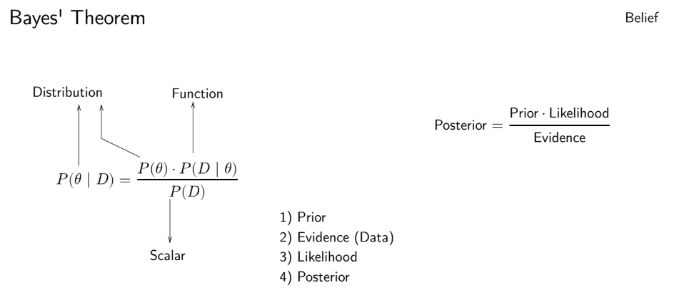
🎯 Bayes’s Theorem

📊 Mean and Mode of Beta Distribution

Mean:
\[ \text{Mean} = \frac{\alpha}{\alpha + \beta} \]
Mode:
\[ \text{Mode} = \begin{cases} \frac{\alpha -1}{\alpha + \beta -2}, & \alpha, \beta \geq 1 \\ 0, & \alpha \leq 1, \, \beta > 1 \\ 1, & \alpha > 1, \, \beta \leq 1 \\ (0, 1), & \alpha = \beta = 1 \\ \{0, 1\}, & \alpha, \beta \leq 1 \end{cases} \]

👉 Note: Most of the time, we use the first case:
\[ \frac{\alpha -1}{\alpha + \beta -2} \]

🔁 Generating Data Points from GMM

The process of generating a data point from a GMM involves two steps:

Choose the component \(k\) by setting \(z_i = k\) with prior probability \(\pi_k\).
Sample a point from the Gaussian associated with this component: \[ \mathcal{N}(x_i; \mu_k, \sigma^2_k) \]

Thus, the joint density of a point \(x_i\) from component \(k\) is:
\[ f(X = x_i, Z = k) = \pi_k \cdot \mathcal{N}(x_i; \mu_k, \sigma^2_k) \]

Marginalizing over \(Z\) gives:
\[ f(X = x_i) = \sum_{k=1}^{K} f(X = x_i, Z = k) \]

Simplified form:
\[ f(X = x_i) = \sum_{k=1}^{K} \pi_k \cdot \mathcal{N}(x_i; \mu_k, \sigma^2_k) \]

👉 This is the density function of the GMM.

📏 Interpretation of \(\lambda^k_i\) (Conditional Probability)

\(i\) represents the index of the data point.
\(k\) represents the component index.
\(\lambda^k_i\) is the conditional probability that the \(i^{\text{th}}\) data point comes from component \(k\), given the data point \(x_i\).

\[ \lambda^k_i = P(z_i = k \mid X = x_i) \]

Using Bayes’ Theorem:
\[ \lambda^k_i = \frac{P(z_i = k) \cdot P(X = x_i \mid z_i = k)}{P(X = x_i)} \]

Substitute with GMM parameters:
\[ \lambda^k_i = \frac{\pi_k \cdot \mathcal{N}(x_i; \mu_k, \sigma^2_k)}{\sum_{j=1}^{K} \pi_j \cdot \mathcal{N}(x_i; \mu_j, \sigma^2_j)} \]

👉 Fact: Since \(\lambda^k_i\) represents probabilities, their sum across all components equals 1:
\[ \sum_{k=1}^{K} \lambda^k_i = 1 \]

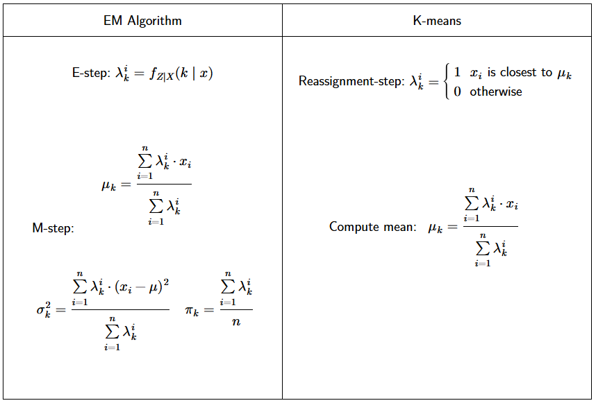
🔄 EM Algorithm Steps

1. Expectation Step (E-Step)

Estimate \(\lambda^k_i\) using the current values of \(\pi_k\), \(\mu_k\), and \(\sigma^2_k\):

\[ \lambda^k_i = \frac{\pi_k \cdot \mathcal{N}(x_i; \mu_k, \sigma^2_k)}{\sum_{j=1}^{K} \pi_j \cdot \mathcal{N}(x_i; \mu_j, \sigma^2_j)} \]

2. Maximization Step (M-Step)

Use the values of \(\lambda^k_i\) obtained in the E-step to update the parameters \(\pi_k\), \(\mu_k\), and \(\sigma^2_k\):

Update Mean \(\mu_k\): \[ \mu_k = \frac{\sum_{i=1}^{n} \lambda^k_i \cdot x_i}{\sum_{i=1}^{n} \lambda^k_i} \]
Update Variance \(\sigma^2_k\): \[ \sigma^2_k = \frac{\sum_{i=1}^{n} \lambda^k_i \cdot (x_i - \mu_k)^2}{\sum_{i=1}^{n} \lambda^k_i} \]
Update mixture probabilities \(\pi_k\): \[ \pi_k = \frac{\sum_{i=1}^{n} \lambda^k_i}{n} \]

💡 EM Algorithm vs. k-Means

💡 Need Help?

For any technical issues or errors, please contact:
📧 22f3001839@ds.study.iitm.ac.in