Week 11 FAQs

📚 Topics Covered in Week 11

• Soft Margin Support Vector Machine (SVM)
• Bias -variance tradeoff
• Ensemble Techniques
  • Bagging
  • Random Forest
  • Adaboost

---

🔍 Soft Margin Support Vector Machine (SVM)

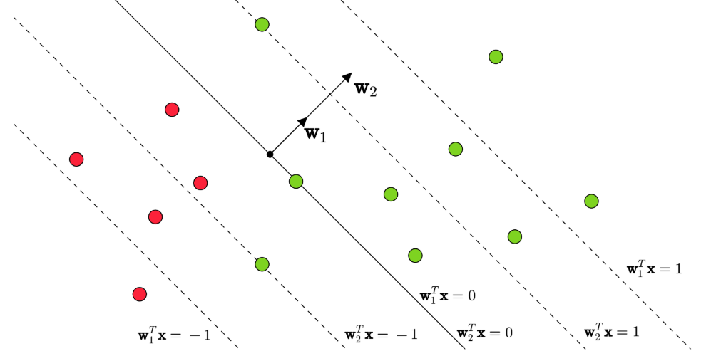
Soft Margin SVM relaxes the condition of perfect linear separability. The separating hyperplane is still defined as:

\[ (\mathbf{w}^T \mathbf{x}_i)y_i = \pm 1 \]

But now, we allow two types of violations:

1. Points are correctly classified but lie inside the margin.
2. Points lie on the wrong side of the hyperplane (misclassified).

To account for these violations, we introduce a non-negative penalty (slack variable) for each point:

\[ \epsilon_i = \max(0, 1 - (\mathbf{w}^T \mathbf{x}_i)y_i) \]

This can be seen as the “cost” for violating the margin or being misclassified.

📏 Constraint Reformulation:

\[ (\mathbf{w}^T \mathbf{x}_i)y_i + \epsilon_i \geq 1, \quad \epsilon_i \geq 0 \]

---

🧠 Optimization Objective

The modified objective balances maximizing margin and minimizing total penalty:

\[ \min_{\mathbf{w}, \ \boldsymbol{\epsilon}} \ \frac{1}{2} \|\mathbf{w}\|^2 + C \cdot \sum_{i=1}^{n} \epsilon_i \]

• The first term encourages a wide margin.
• The second penalizes violations.
• \(C\) is a hyperparameter that controls the trade-off.

By substituting the slack expression, we obtain the Hinge Loss form:

\[ \min_{\mathbf{w}} \ \frac{1}{2} \|\mathbf{w}\|^2 + C \cdot \sum_{i=1}^{n} \max\left(0, 1 - (\mathbf{w}^T \mathbf{x}_i)y_i\right) \]

This reflects the balance between margin width and classification error.

🔁 Trade-off Insights

• Smaller \(\|\mathbf{w}\|\) → wider margin → more violations (higher loss).
• Larger \(\|\mathbf{w}\|\) → smaller margin → fewer violations.
• Small \(C\): prioritizes margin over misclassification.
• Large \(C\): prioritizes minimizing misclassification, similar to hard-margin SVM.

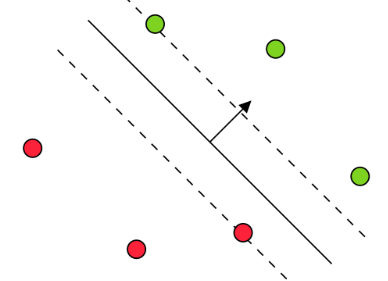
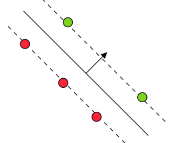
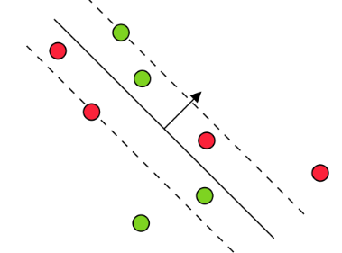
📈 Visual Representation:

---

🔧 Solving the Optimization

\[ \min_{\mathbf{w}, \epsilon} \ \frac{\|\mathbf{w}\|^2}{2} + C \sum_{i=1}^{n} \epsilon_i \] \[ \text{ subject to: } (\mathbf{w}^T \mathbf{x}_i)y_i + \epsilon_i \geq 1, \ \epsilon_i \geq 0 \]

Primal Formulation:

By introducing Lagrange multipliers:

• \(\alpha_i\) for the margin constraint
• \(\beta_i\) for the non-negativity of \(\epsilon_i\)

\[ \min_{\mathbf{w}, \mathbf{\xi}} \quad \max_{\mathbf{\alpha} \geq 0, \mathbf{\beta} \geq 0} \quad \frac{\|\mathbf{w}\|^2}{2} + C \cdot \sum_{i=1}^{n} \xi_i + \sum_{i=1}^{n} \alpha_i \left( 1 - (\mathbf{w}^T \mathbf{x}_i) y_i - \xi_i \right) - \sum_{i=1}^{n} \beta_i \xi_i \]

Dual Formulation:

From the primal, we derive the dual problem

\[ \max_{\mathbf{\alpha} \geq 0, \mathbf{\beta} \geq 0} \quad \min_{\mathbf{w}, \mathbf{\xi}} \quad \frac{\|\mathbf{w}\|^2}{2} + C \cdot \sum_{i=1}^{n} \xi_i + \sum_{i=1}^{n} \alpha_i \left( 1 - (\mathbf{w}^T \mathbf{x}_i) y_i - \xi_i \right) - \sum_{i=1}^{n} \beta_i \xi_i \]

Solving the dual gives:

\[ \mathbf{w} = \sum_{i=1}^n \alpha_i y_i \mathbf{x}_i \quad \text{and} \quad \alpha_i + \beta_i = C \]

Final dual objective:

\[ \max_{0 \leq \alpha \leq C} \ \alpha^T \mathbf{1} - \frac{1}{2} \alpha^T (Y^T X^T X Y) \alpha \]

Compared to the hard-margin version, the only change is the upper bound on \(\alpha_i\):

• Hard margin: \(\alpha_i \in [0, \infty)\)
  
• Soft margin: \(\alpha_i \in [0, C]\)

---

⭐ Support Vectors

Support vectors are data points for which \(\alpha^* > 0\). They are crucial in defining the decision boundary.

Complemnetary slackness condition:

This principle states: if a constraint is not active, its corresponding multiplier is zero.

Primal constraints

\[ \epsilon_i^* \geq 0, \quad (\mathbf {w^*}^T\mathbf x_i)y_i + \epsilon_i^* \geq 1 \]

We also know:

\[ \epsilon_i^* = \max (0, 1-(\mathbf {w^*}^T\mathbf x_i)y_i) \]

Dual Constraint:

\[ \alpha_i^* \geq 0, \ \beta_i^* \geq 0, \ \alpha_i^* + \beta_i^* = C \]

For optimal values \(\alpha_i^*\), \(\beta_i^*\), \(\xi_i^*\), we have the following complemnetary slackness conditions:

\[ \alpha_i^* \cdot [1 - y_i(\mathbf{w}^T \mathbf{x}_i) - \xi_i^*] = 0, \quad \beta_i^* \cdot \xi_i^* = 0 \]

This gives a precise classification of points:

---

🔍 Primal View

Type	Condition	Mathematical Form	Properties	Example
Not Support Vectors	Outside margin	\((\mathbf{w}^T \mathbf{x}_i)y_i > 1\)	\(\xi_i^* = 0, \alpha_i^* = 0\)
Possible Support Vectors	On margin	\((\mathbf{w}^T \mathbf{x}_i)y_i = 1\)	\(\xi_i^* = 0, \alpha_i^* \in [0, C]\)
Support Vectors	Inside margin or misclassified	\((\mathbf{w}^T \mathbf{x}_i)y_i < 1\)	\(\xi_i^* > 0, \alpha_i^* = C\)

---

🔁 Dual View

\(\alpha_i^*\)	Condition	Properties	Example
\(= 0\)	\(\xi_i^* = 0, (\mathbf{w}^T \mathbf{x}_i)y_i \geq 1\)	Not support vectors
\(\in (0, C)\)	\(\xi_i^* = 0, (\mathbf{w}^T \mathbf{x}_i)y_i = 1\)	Support vectors on margin
\(= C\)	\(\xi_i^* \geq 0, (\mathbf{w}^T \mathbf{x}_i)y_i \leq 1\)	Key support vectors

---

🔍 Bias-Variance Trade-off

• Bias: Measures the accuracy of the predictions — how close the model’s outputs are to the true values. Lower error implies lower bias. Generally, as the complexity of the model increases, bias tends to decrease. High-bias models tend to underfit the data.

• Variance: Measures the sensitivity of the model to fluctuations in the training data. As model complexity increases, variance also increases. High-variance models tend to overfit the training data.

---

🔍 Ensemble Techniques

Ensemble methods combine multiple simple models (often called weak learners) to build a stronger, more robust model. Individually, these models might perform only slightly better than random guessing, but when combined, they can deliver powerful predictions.

• Ensemble methods distribute the prediction task across multiple weak learners.
• How can we ensure diversity among these learners?
• Why does combining multiple models lead to better performance?

Why Do Ensembles Work?

Let’s understand this with a bit of probability theory.
Assume we have \(n\) independent, identically distributed (i.i.d.) random variables \(X_i\), where:

\[ Var(X_i) = \sigma^2 \]

The variance of their mean is:

\[ Var\left(\overline{X}\right) = Var\left(\frac{1}{n} \sum_{i=1}^{n} X_i\right) = \frac{1}{n^2} \sum_{i=1}^{n} Var(X_i) = \frac{1}{n^2} \cdot n \sigma^2 = \frac{\sigma^2}{n} \]

Note: This simplification relies on the i.i.d. assumption. \(Var(A+B) = Var(A) + Var(B)\) is not always possible.

Takeaway:

• Averaging reduces variance!
  
• Although we usually have only one dataset, we can mimic multiple datasets by creating “bootstrap” samples.

Bagging

Bagging stands for Bootstrap Aggregating.

Process:

1. Bootstrap Sampling:
   Create multiple “bags” by randomly sampling the dataset with replacement.
   Probability that a data point appears in at least one bag:

   \[ 1 - \left(1 - \frac{1}{n}\right)^n \approx 63\% \]

2. Model Training:
   Train a separate model (base learner) on each bag.

3. Prediction:

   • Regression: Take the average of predictions:

     \[ \frac{1}{B} \sum_{b=1}^{B} \hat{f}^{b}(x) \]

   • Classification: Take the majority vote:

     \[ \text{Majority Vote} \left\{\hat{f}^b(x)\right\}_{b=1}^{B} \]

Observations:

• Bagging can be parallelized.
• Any model can be used as a base learner.
• However, interpretability is reduced compared to a single decision tree.

---

Random Forest

In certain scenarios, bagged trees can become highly correlated.
For example, consider a dataset that contains one dominant feature alongside several moderately important ones. During training, each decision tree in the bagging ensemble is likely to select this dominant feature for its top-level split. As a result, many of the trees end up looking very similar, making their predictions closely correlated.

Now, here’s the issue:
Averaging highly correlated predictions does not significantly reduce variance. The benefit of bagging relies on diversity among the base learners. If all the trees make similar errors, averaging them does little to improve performance. In such cases, bagging may not provide a meaningful variance reduction compared to using a single decision tree.

🌟 Why Does This Matter?

The main goal of bagging is to reduce variance by combining many different models.
However, if the models are too similar, they make similar mistakes.
It’s like asking the same group of friends (who all think alike) for advice — you won’t get fresh perspectives!
By decorrelating the trees, we ensure they capture different patterns in the data. This leads to a stronger, more reliable ensemble that better generalizes to unseen data.

Random Forest addresses this by adding an extra layer of randomness:

• At each split in the tree, it considers only a random subset of features.

• If there are \(d\) total features, we randomly select \(m\) features at each split, where typically:

  \[ m \approx \sqrt{d} \]

This strategy decorrelates the trees, improving variance reduction and leading to a more reliable ensemble.

Boosting

While bagging reduces variance, boosting focuses on reducing bias. Boosting builds models sequentially, where each new model attempts to correct the errors of its predecessor.

AdaBoost

Process:

1. Initialize weights:
   Assign equal weight to all data points:

   \[ D_0(i) = \frac{1}{n} \]

2. For each round \(t = 1, 2, \dots, T\):

   • Train weak classifier \(h_t\) on data weighted by \(D_{t-1}\).

   • Compute weighted error:

     \[ \epsilon_t = \sum_{i=1}^{n} D_{t-1}(i) \cdot \mathbf{1}_{\{y_i \neq h_t(\mathbf{x}_i)\}} \]

   • Compute model weight:

     \[ \alpha_t = \frac{1}{2} \ln \left( \frac{1 - \epsilon_t}{\epsilon_t} \right) \]

   • Update data weights:

     \[ \tilde{D}_t(i) = \begin{cases} e^{\alpha_t} \cdot D_{t-1}(i) & \text{if } h_t(\mathbf{x}_i) \neq y_i \\ e^{-\alpha_t} \cdot D_{t-1}(i) & \text{if } h_t(\mathbf{x}_i) = y_i \end{cases} \]

     Normalize:

     \[ D_t(i) = \frac{\tilde{D}_t(i)}{\sum_{j=1}^{n} \tilde{D}_t(j)} \]

3. Final prediction:

   \[ \operatorname{sign} \left( \sum_{t=1}^{T} \alpha_t h_t(\mathbf{x}_i) \right) \]

Observations:

• Boosting trains models sequentially, focusing on correcting previous mistakes.
• Unlike bagging, boosting can overfit if the number of rounds \(T\) is too large, but this typically happens slowly.
• Weaker classifiers are assigned higher weights in the ensemble.
• Final prediction is a weighted sum of individual classifiers, prioritizing better-performing models.

---

💡 Need Assistance?

📧 22f3001839@ds.study.iitm.ac.in

---

⬅️ Week 10

Week 12 ➡️