Week 6 FAQs
📚 Topics Covered in Week 6
- Goodness of Maximum Likelihood Estimation (MLE) in Linear Regression
- Ridge Regression
- Lasso Regression
- Cross-Validation Techniques
- Probabilistic Interpretation
- Geometric Perspective
- Model Complexity and Generalization
🔍 Goodness of Maximum Likelihood Estimation (MLE) in Linear Regression
The maximum likelihood estimate (MLE) of the true weight vector \(\mathbf{w}\), denoted as \(\mathbf{\hat{w}}\), is given by:
\[ \mathbf{\hat{w}} = (\mathbf{XX}^T)^{\dagger}\mathbf{Xy} \]
Assuming that for a given data point \(\mathbf{x}_i\), we have:
\[ y_i = \mathbf{w}^T\mathbf{x}_i + \epsilon_i, \quad \text{where } \epsilon_i \sim \mathcal{N}(0, \sigma^2) \]
Treating \(\mathbf{x}_i\) as fixed and \(y_i\) as a random variable, its conditional distribution follows:
\[ y_i \mid \mathbf{x}_i \sim \mathcal{N}(\mathbf{w}^T\mathbf{x}_i, \sigma^2) \]
For a dataset with \(n\) observations, we can express the conditional distribution of the response vector as:
\[ \mathbf{y} \mid \mathbf{X} \sim \mathcal{N}(\mathbf{X}^T\mathbf{w}, \sigma^2 \mathbf{I}) \]
Since \(\mathbf{y}\) is a random vector, \(\mathbf{\hat{w}}\) is also a random vector. To evaluate how close \(\mathbf{\hat{w}}\) is to \(\mathbf{w}\) on average, we examine the expected squared error:
\[ E\left[ \| \mathbf{w} - \mathbf{\hat{w}} \|^2\right] = \sigma^2 \cdot \text{trace}\left[(\mathbf{XX}^T)^{-1}\right] = \sigma^2 \cdot \sum_{i=1}^n \cfrac{1}{\lambda_i} \]
where \(\lambda_i\) denotes the eigenvalues of \((\mathbf{XX}^T)^{-1}\). This suggests that the mean squared error (MSE) depends on:
- The variance of the noise term \(\epsilon\)
- The trace of \((\mathbf{XX}^T)^{-1}\)
While we cannot control the variance of \(\epsilon\), we can influence the trace component by introducing regularization:
\[ \mathbf{\hat{w}}_{\text{new}} = (\mathbf{XX}^T + \lambda \mathbf{I})^{-1}\mathbf{Xy} \]
where the modified eigenvalues become:
\[ \sum_{i=1}^n \frac{1}{\lambda_i + \lambda} \]
This modification reduces the MSE compared to the standard MLE approach.
🔍 Ridge Regression
Ridge regression introduces a regularization term to the loss function, modifying it as follows:
\[ L(\mathbf{w}) = \frac{1}{2} \sum_{i=1}^{n} \left( \mathbf{w}^T \mathbf{x}_i - y_i \right)^2 + \frac{\lambda}{2} \|\mathbf{w}\|_2^2 \]
where the \(L_2\) norm is defined as:
\[ \|\mathbf{w}\|_2^2 = w_1^2 + w_2^2 + \cdots + w_d^2 \]
The regularization parameter \(\lambda\) controls the trade-off between model complexity and bias. Ridge regression shrinks the weight coefficients toward zero but does not set them exactly to zero. The optimal weight vector is given by:
\[ \mathbf{\hat{w}} = (\mathbf{XX}^T + \lambda \mathbf{I})^{-1} \mathbf{Xy} \]
Keep in mind that the weight vector \(\mathbf{\hat{w}}\) is identical to the one derived in the Goodness of Maximum Likelihood Estimation (MLE) in Linear Regression section.
🔍 Lasso Regression
Lasso regression (Least Absolute Shrinkage and Selection Operator) modifies the loss function by introducing an \(L_1\) penalty:
\[ L(\mathbf{w}) = \frac{1}{2} \sum_{i=1}^{n} \left( \mathbf{w}^T \mathbf{x}_i - y_i \right)^2 + \lambda \|\mathbf{w}\|_1 \]
where the \(L_1\) norm is given by:
\[ \|\mathbf{w}\|_1 = |w_1| + |w_2| + \cdots + |w_d| \]
Unlike Ridge regression, Lasso can drive some coefficients to exactly zero, resulting in sparse solutions. However, there is no closed-form solution for Lasso regression.
🔍 Cross-Validation
To determine the optimal value of \(\lambda\), we use cross-validation techniques:
K-Fold Cross-Validation
The dataset is partitioned into \(k\) folds, with \(k-1\) folds used for training and the remaining fold for validation. This process is repeated until each fold has served as the validation set.
Leave-One-Out Cross-Validation (LOOCV)
Each data point serves as a validation sample while the rest form the training set. This method is computationally expensive but useful for small datasets.
🔍 Probabilistic Perspective
In the previous discussion, we estimated the parameter vector \(\mathbf{w}\) using Maximum Likelihood Estimation (MLE). Now, we adopt a Bayesian approach for parameter estimation.
Bayesian Estimation
According to Bayes’ theorem, the posterior distribution is proportional to the product of the prior distribution and the likelihood function:
\[ \text{Posterior} \propto \text{Prior} \times \text{Likelihood} \]
Prior Distribution
We assume a Gaussian prior on \(\mathbf{w}\):
\[ \mathbf{w} \sim \mathcal{N}(\mathbf{0}, \gamma^2 \mathbf{I}) \]
This represents a multivariate normal distribution with a mean vector of zero and an isotropic covariance matrix. Given the independence of the components of \(\mathbf{w}\), we can express the prior distribution as a product of \(d\) univariate Gaussians:
\[ \begin{array}{l} P(\mathbf{w}) \propto \exp\left[\frac{-( w_{1} -0)^{2}}{2\gamma ^{2}}\right] \cdots \exp\left[\frac{-( w_{d} -0)^{2}}{2\gamma ^{2}}\right]\\ \\ P(\mathbf{w}) \propto \exp\left[\frac{-\sum\limits _{i=1}^{d} w_{i}^{2}}{2\gamma ^{2}}\right] \end{array} \]
Likelihood Function
Given that the observed outputs \(y_i\) follow a normal distribution:
\[ y_i \sim \mathcal{N}(\mathbf{w}^T \mathbf{x}, \sigma^2) \]
The likelihood function for the dataset \(D\) is given by:
\[ P(D \mid \mathbf{w}) \propto \prod _{i=1}^{n}\exp\left[\frac{- ( y_{i} - \mathbf{w}^{T}\mathbf{x}_{i})^{2}}{2\sigma ^{2}}\right] \]
Posterior Distribution and MAP Estimation
Taking the logarithm of the posterior and simplifying by removing constants, we obtain:
\[ -\sum _{i=1}^{n}\frac{( y_{i} - \mathbf{w}^{T}\mathbf{x}_{i})^{2}}{2\sigma ^{2}} - \frac{\sum\limits _{j=1}^{d} w_{j}^{2}}{2\gamma ^{2}} \]
To estimate \(\mathbf{w}\), we maximize the posterior, which is equivalent to the Maximum A Posteriori (MAP) estimation. By multiplying the MAP objective by \(-1\), we obtain the regularized loss function for ridge regression:
\[ L(\mathbf{w}) = \sum _{i=1}^{n}\frac{( y_{i} - \mathbf{w}^{T}\mathbf{x}_{i})^{2}}{2\sigma ^{2}} + \frac{1}{2\gamma ^{2}} \| \mathbf{w} \| _{2}^{2} \]
Key Insights
- The MAP estimate under a zero-mean Gaussian prior coincides with the ridge regression solution.
- The MAP estimate under a zero-mean Laplacian prior corresponds to the LASSO regression solution.
🔍 Geometric Interpretation
Minimizing Ridge loss is equivalent to solving:
\[ \min_{\mathbf{w}} \frac{1}{2} \sum_{i=1}^{n} \left( \mathbf{w}^T \mathbf{x}_i - y_i \right)^2 \]
subject to:
\[ \|\mathbf{w}\|_2^2 \leq \theta \]
where \(\theta\) is some scalar dependent on \(\lambda\).
The constraint forces weight values to remain within a bounded region. Lasso imposes an \(L_1\) constraint, which often results in sparse solutions.
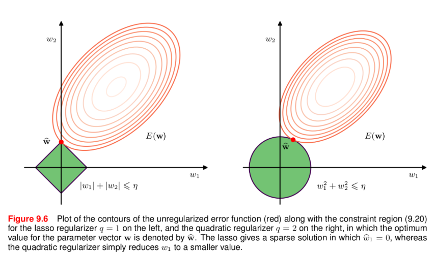
Left one is Lasso and right one is Ridge.
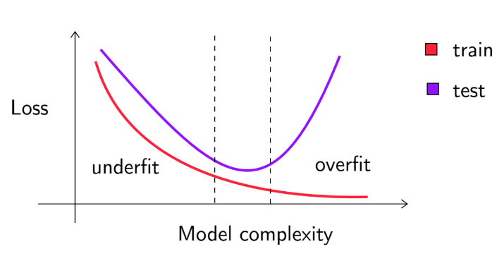
🔍 Model Complexity and Generalization
A balance between model complexity and generalization is essential. If training loss is low but test loss is high, the model overfits. If both losses are high, the model underfits. The relationship is illustrated below:
💡 Need Assistance?
For any technical queries, feel free to reach out via email: 📧 22f3001839@ds.study.iitm.ac.in