Week 8 FAQs
📚 Topics Covered in Week 8
- Discriminative vs. Generative Models
- Generative Models
- Naive Bayes
- Linear Discriminant Analysis (Gaussian Naive Bayes)
🔍 Discriminative vs. Generative Models
Generative Models
A generative model learns the joint probability distribution between features and labels:
\[ P(\mathbf{x} \mid y) = P(y) \cdot P(\mathbf{x} \mid y) \]
It aims to understand how the data is generated by estimating \(P(\mathbf{x} \mid y)\), which can then be used to infer \(P(y \mid \mathbf{x})\) via Bayes’ rule. Generative models perform well when the chosen distribution closely aligns with the true data-generating process.
Discriminative Models
A discriminative model directly estimates the conditional probability \(P(y \mid \mathbf{x})\), focusing solely on classifying a given example \(\mathbf{x}\) into a class \(y\). These models do not attempt to model how the data was generated but instead focus on distinguishing between different classes.
| Discriminative Model | Generative Model | |
|---|---|---|
| Objective | Directly estimate \( P(y|x) \) | Estimate \( P(x|y) \) and deduce \( P(y|x) \) |
| Learning Focus | Decision boundary | Probability distributions of data |
| Illustration | 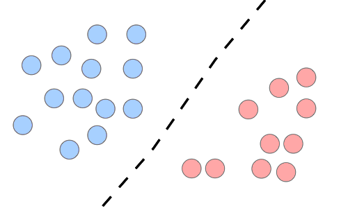 |
 |
| Examples | Regression models, SVMs | GDA, Naive Bayes |
🔍 Generative Models
Parameter Calculation
Case 1: No Class-Conditional Independence Assumption
If we have \(C\) classes and features that take values in \(\{0, \dots, k-1\}\), i.e.,
\[ \mathbf{x}_i \in \{0, \dots, k-1\}^d, \quad y_i \in \{1, \dots, C\} \]
The number of free parameters is computed as follows:
- \(C-1\) parameters for the class probabilities (since the last probability can be inferred).
- For each class, the feature combinations total \(k^d\). Using the probability sum rule, the number of free parameters per class is \(k^d - 1\).
- Since we compute this for all \(C\) classes, the total number of parameters is:
\[ C \times (k^d - 1) + (C - 1) \]
For binary classification with binary features:
\[ 2 \times (2^d -1) + 1 \]
Case 2: Class-Conditional Independence Assumption
In this case, we assume independence among features given the class:
\[ C \times d(k-1) + (C-1) \]
For binary classification with binary features:
\[ 2d + 1 \]
🔍 Naive Bayes
For binary features and binary classification:
\[ \mathbf{x}_i \in \{0,1\}^d, \quad y_i \in \{0,1\} \]
The prior probability of the label is estimated as:
\[ p= P(Y=1) = \cfrac{\sum\limits _{i=1}^{n}\mathbb{I}( y_{i} =1)}{n} \]
The conditional probability for feature \(j\) given class \(y\) is:
\[ p^y_j = P(X_j=1 \mid Y=y) = \cfrac{\sum\limits _{i=1}^{n}\mathbb{I}( y_{i} =y)\mathbf{x}_{ij}}{\sum\limits _{i=1}^{n}\mathbb{I}( y_{i} =y)} \]
Laplace Smoothing
To prevent zero probabilities, we use Laplace smoothing by adding pseudo-counts:
- If \(p^y_j = 0\), add a data point where all features are 1.
- If \(p^y_j = 1\), add a data point where all features are 0.
This results in four additional data points (two per class), modifying the estimates accordingly.
Prediction
Using Bayes’ rule:
\[ P( y=1 \mid \mathbf{x}_{\text{test}}) = \cfrac{P( y=1) P(\mathbf{x}_{\text{test}} \mid y=1)}{P(\mathbf{x}_{\text{test}})} \]
\[ P( y=0 \mid \mathbf{x}_{\text{test}}) = \cfrac{P( y=0) P(\mathbf{x}_{\text{test}} \mid y=0)}{P(\mathbf{x}_{\text{test}})} \]
If only classification is required:
\[ \hat{y} = \begin{cases} 1 & P( y=1) P(\mathbf{x}_{\text{test}} \mid y=1) \geq P( y=0) P(\mathbf{x}_{\text{test}} \mid y=0) \\ 0 & \text{otherwise} \end{cases} \]
Naive Bayes has a linear decision boundary.
🔍 Linear Discriminant Analysis (Gaussian Naive Bayes)
LDA assumes that data within each class follows a multivariate Gaussian distribution with a shared covariance matrix:
\[ \mathbf{x} \mid y = 0 \sim \mathcal{N}(\mathbf{\mu}_0, \mathbf{\Sigma}) \] \[ \mathbf{x} \mid y = 1 \sim \mathcal{N}(\mathbf{\mu}_1, \mathbf{\Sigma}) \]
Using MLE, we estimate:
\[ \mathbf{\mu}_1 = \cfrac{\sum\limits _{i=1}^{n}\mathbb{I}( y=1)\mathbf{x}_{i}}{\sum\limits _{i=1}^{n}\mathbb{I}( y=1)} , \quad \mathbf{\mu}_0 = \cfrac{\sum\limits _{i=1}^{n}\mathbb{I}( y=0)\mathbf{x}_{i}}{\sum\limits _{i=1}^{n}\mathbb{I}( y=0)} \]
\[ \mathbf{\Sigma} = \cfrac{1}{n} \sum _{i=1}^{n}(\mathbf{x}_{i} -\mathbf{\mu}_{y_{i}})(\mathbf{x}_{i} -\mathbf{\mu}_{y_{i}})^{T} \]
LDA also has a linear decision boundary.
💡 Need Assistance?
For any technical queries, feel free to reach out via email: 📧 22f3001839@ds.study.iitm.ac.in