Week 5 FAQs
📚 Topics Covered in Week 5
- Supervised Learning
- Regression
- Classification
- Linear Regression
- Simple Linear Model
- Normal Equation
- Gradient Descent
- Stochastic Gradient Descent (SGD)
- Kernel Regression
- Probabilistic Perspective
🔍 Visualization of Linear Regression
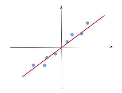
Linear regression is a fundamental statistical method that models the relationship between input features and a target variable by fitting a linear function. It assumes a linear correlation between data points and their corresponding labels.
Single Feature Regression
Two Features Regression
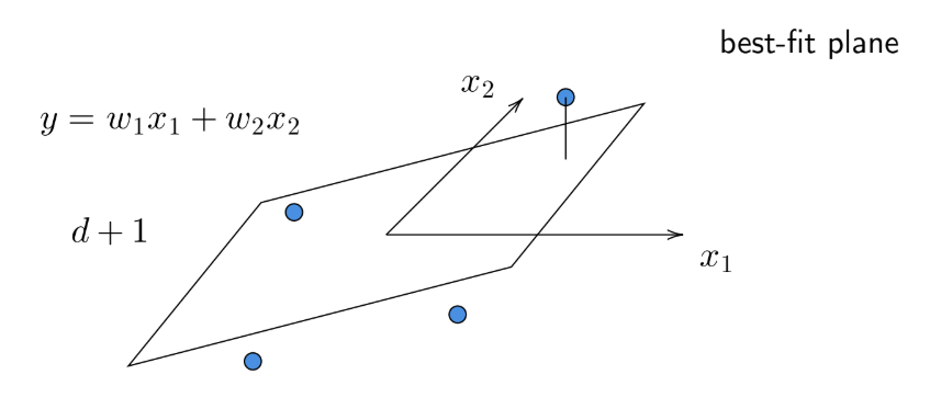
For a dataset in \(\mathbb{R}^d\), the best-fit hyperplane describing the linear relationship lies in \(\mathbb{R}^{d+1}\).
🔍 Performance Metrics
For a given dataset, where \(\mathbf{x}_i\) represents the data point and \(y_i\) is the corresponding true label, we define the following error metrics:
Sum of Squared Errors (SSE) \[ \text{SSE} = \sum_{i=1}^{n} \left[f(\mathbf{x}_i) - y_i \right]^2 \]
Mean Squared Error (MSE) \[ \text{MSE} = \frac{1}{n} \sum_{i=1}^{n} \left[f(\mathbf{x}_i) - y_i \right]^2 \]
Root Mean Squared Error (RMSE) \[ \text{RMSE} = \sqrt{\frac{1}{n} \sum_{i=1}^{n} \left[f(\mathbf{x}_i) - y_i \right]^2} \]
🔍 Normal Equation
The Normal Equation provides a closed-form solution to the least squares problem. For a data matrix \(\mathbf{X}\) of shape \(d \times n\):
\[ \hat{\mathbf{w}} = \left(\mathbf{XX}^T\right)^{\dagger} \mathbf{Xy} \]
where \((\mathbf{XX}^T)^{\dagger}\) represents the Moore–Penrose inverse and \(\mathbf{y}\) is the true label vector.
If \(\mathbf{XX}^T\) is invertible then
\[ \hat{\mathbf{w}} = \left(\mathbf{XX}^T\right)^{-1} \mathbf{Xy} \]
For a single-feature case, the simplified form is:
\[ \hat{\mathbf{w}} = \frac{\sum^{n}_{i=1} \mathbf{x}_i y_i}{\sum^{n}_{i=1} \mathbf{x}_i^2} \]
🔍 Gradient Descent Method
Computing the Moore-Penrose inverse is computationally expensive for large datasets. Instead, Gradient Descent provides an iterative optimization approach to minimize the error function.
The gradient of SSE is given by:
\[ \nabla L(\mathbf{w}) = 2[\mathbf{XX}^T\mathbf{w} - \mathbf{Xy}] \]
The weight update rule is:
\[ \mathbf{w}^{t+1} = \mathbf{w}^{t} - \eta \nabla{L(\mathbf{w})} \]
where \(L\) represents the loss function, and \(\eta\) is the learning rate.
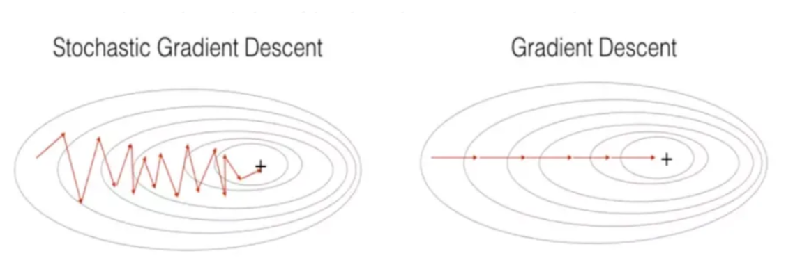
🔍 Stochastic Gradient Descent (SGD)
For large datasets, computing gradients over the entire dataset can be expensive. SGD mitigates this by computing gradients using a randomly selected subset of data at each iteration.
📺 Watch this video for a detailed explanation: SGD vs GD
⚠️ Note: As SGD updates based on small subsets, it introduces more variance during convergence, as visualized below:
🔍 Geometric Perspective
Our objective is to find \(\mathbf{w}\) such that:
\[ \mathbf{X}^T \mathbf{w} \approx \mathbf{y} \]
From a geometric viewpoint, \(\mathbf{X}^T \mathbf{w}\) represents a linear combination of feature vectors. The projection of \(\mathbf{y}\) onto the plane spanned by the columns of \(\mathbf{X}^T\) gives the best approximation.
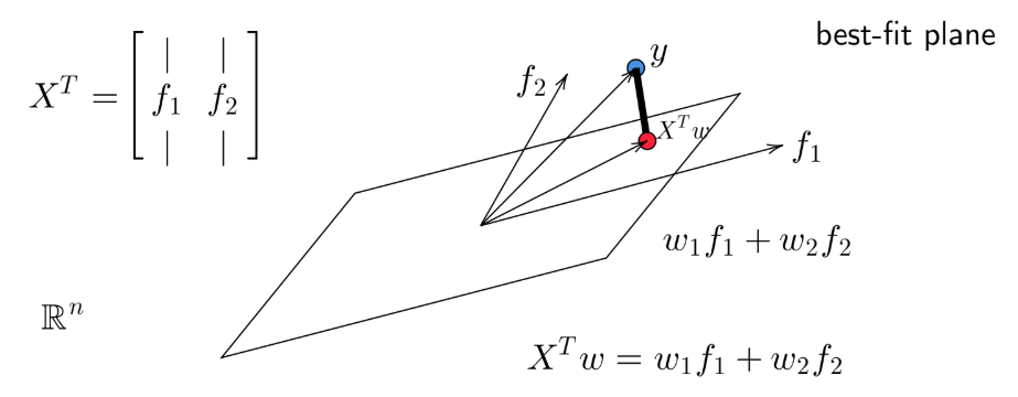
This naturally leads back to the Normal Equation formulation.
🔍 Kernel Regression
For non-linear relationships, the weight vector is defined as:
\[ \hat{w} = \phi(\mathbf{X})\alpha \]
where \(\alpha = \mathbb{K}^{\dagger} y\).
Prediction Formula:
\[ \hat{y} = \sum^{n}_{i=1} \hat{\alpha_i} \cdot k(\mathbf{x}_\text{test}, \mathbf{x}_i) \]
- \(\alpha_i\) represents the importance of the \(i^{\text{th}}\) data point in predicting the label.
- \(k(\mathbf{x}_\text{test}, \mathbf{x}_i)\) measures similarity between the test and training data points.
🔍 Probabilistic Perspective
We assume that each label is generated by adding noise to the true relationship:
\[ y_i = \mathbf{w}^T \mathbf{x}_i + \epsilon_i \]
where \(\epsilon_i \sim \mathcal{N}(0, \sigma^2)\), leading to:
\[ y_i \mid x_i \sim \mathcal{N}(0, \sigma^2) \]
Using Maximum Likelihood Estimation (MLE), we derive:
\[ \min_{w} \sum_{i=1}^{n} (y_i - \mathbf{w}^T\mathbf{x}_i)^2 \]
which coincides with minimizing SSE. This equivalence holds under a Gaussian noise assumption. If we assume a Laplace distribution, minimizing SSE is replaced by minimizing the absolute error, which leads to a robust regression technique. Read more on Laplace distribution applications.
💡 Need Help?
For technical queries, feel free to reach out via email: 📧 22f3001839@ds.study.iitm.ac.in