Week 7 FAQs
📚 Topics Covered in Week 7
- Classification
- K-Nearest Neighbors (KNN)
- Decision Trees
🔍 Classification Problems
Given a dataset:
\[D = \left\{ (x_1, y_1), \cdots, (x_n,y_n) \right\}\]
In a regression problem, the labels are continuous values: \(y_i \in \mathbb{R}\). However, in classification, labels belong to a discrete set: \(y_i \in K\), where \(K\) represents the number of classes. For binary classification, \(K=2\).
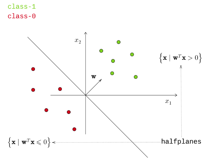
Linear Classifier
A linear classifier employs a line or hyperplane to separate data points into classes. The misclassification loss is defined as:
\[ \frac{1}{n} \sum_{i=1}^{n} \mathbf{1}[h(\mathbf x_i) \neq y_i] \]
where:
\[ h(\mathbf x_i) = \mathfrak{sign}(\mathbf w^T \mathbf x) = \begin{cases} 1 & \mathbf{w}^{T}\mathbf{x} \geqslant 0\\ 0 & \mathbf{w}^{T}\mathbf{x} < 0 \end{cases} \]
By convention in the lectures, a tie-breaking rule assigns \(\mathbf w^T \mathbf x=0\) to class 1. However, this is not a fixed rule and may vary depending on the problem context.
Why Not Use Regression Loss for Classification?
The optimal weight vector \(\mathbf{w}^{\star}\) in regression is obtained by minimizing the squared error loss:
\[ \mathbf{w}^{\star} = \underset{\mathbf w}{{\arg \min}} \frac{1}{n} \sum_{i=1}^{n} (\mathbf w^T \mathbf x-y_i)^2 \]
However, regression loss is not suitable for classification due to the following reasons:
- Sensitivity to Outliers: Regression methods can be significantly affected by extreme values.
- No Natural Ordering: Classification problems involve discrete labels without an inherent order, whereas regression inherently assumes a continuous ordering.
🔍 K-Nearest Neighbors (KNN)
An odd value for \(k\) is typically chosen to avoid ties.
Key hyperparameters:
- \(k\)
- Distance metric:
- \(L_1\) (Manhattan distance)
- \(L_2\) (Euclidean distance)
As \(k\) increases, the model becomes less flexible. A higher \(k\) results in a smoother decision boundary but may fail to capture finer patterns.
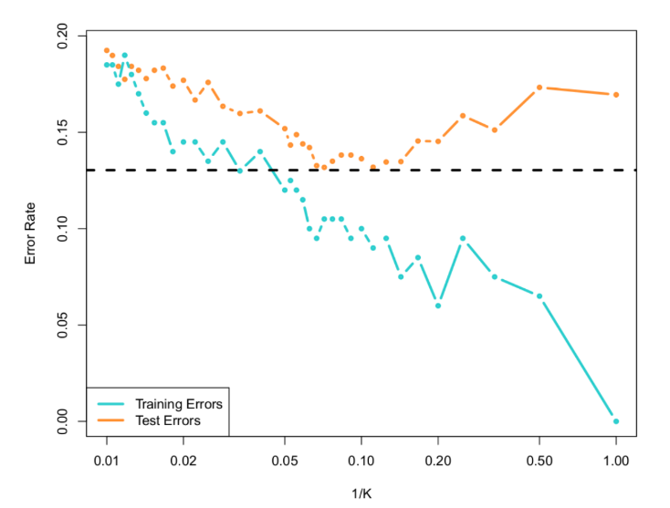

With \(k=1\), KNN can achieve zero misclassification error on the training dataset, considering that a data point is a neighbor of itself.
Curse of Dimensionality: As the number of dimensions increases, distance metrics become less reliable in defining neighborhoods. This significantly impacts KNN’s effectiveness. For further insights, visit this discussion. (It is not discussed in the lectures though but important from learning point of view)
🔍 Decision Trees
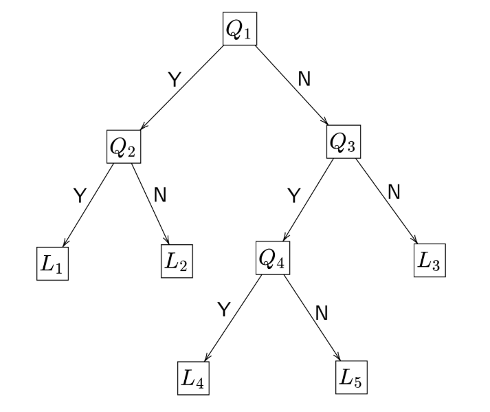
- Nodes:
- Root node: \(Q_1\)
- Internal nodes: \(Q_2, Q_3, Q_4\)
- Leaf nodes: \(L_1, L_2, L_3, L_4, L_5\)
Entropy: A Measure of Impurity
- \(n_P\): Number of positive data points
- \(n_N\): Number of negative data points
\[ n = n_P + n_N \]
- \(p\): Proportion of positive (or negative) data points in a node
\[ p = \frac{n_P}{n} \]
The entropy is given by:
\[ H(p) = -p\log_2p - (1-p)\log_2(1-p) \]
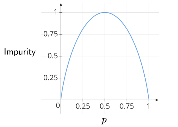
Entropy is symmetric, meaning the result remains unchanged whether we define \(p\) as the proportion of positive or negative samples.
Note: In a pure leaf, all samples belong to the same class, so the impurity (entropy) would be 0.
Information Gain
Information gain is a measure of how much information is gained by splitting a set into subsets.
- \(\gamma\): Proportion of data points going to the left node (L)
- \(n_L\): Number of data points in the left node (L)
- \(n_R\): Number of data points in the right node (R)
- \(E_P\): Entropy of the parent node (P)
- \(E_L\): Entropy of the left node (L)
- \(E_R\): Entropy of the right node (R)
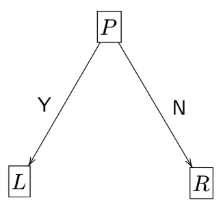
\[ n = n_L + n_R \]
\[ \gamma = \frac{n_L}{n} \]
\[ IG = E_P - [\gamma E_L + (1-\gamma) E_R] \]
Key Properties of Decision Trees:
- Can achieve zero misclassification error on the training dataset.
- Highly sensitive to small changes in the training data, leading to high variance.
- Overfitting is a common issue, especially in deep trees.
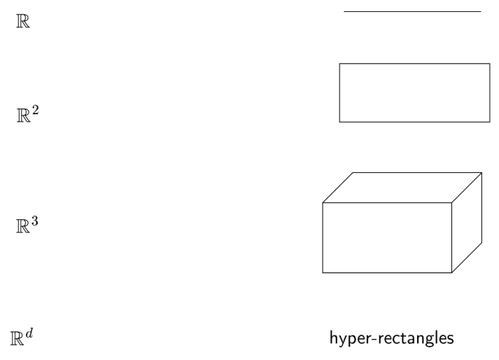
- To create a bounded region in \(d\) dimensions, the tree depth must be at least \(2d\). In general, boundaries of the regions are parallel to the axes:
💡 Need Assistance?
For any technical queries, feel free to reach out via email: 📧 22f3001839@ds.study.iitm.ac.in